15. Polar Coordinates

b.1. Graphs of Polar Equations

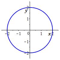
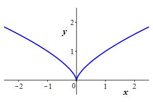
The rectangular graph of an equation is the set of points whose rectangular coordinates, \((x,y)\), satisfy the equation. For example, the graphs of \(x^2+y^2=4\) and \(x^2=y^3\) are

This plot shows a circle of radius 2 centered at the origin. — \(x^2+y^2=4\)

This plot shows a curve which is symmetric across the y axis in the
upper half plane. It starts with a sharp cusp at the origin and rises on both
the left and right sides and is concave down. — \(x^2=y^3\)

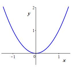
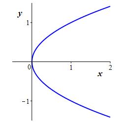
In particular, the graph of a function is the graph of the equation which defines the function. For most purposes, we take \(x\) as the independent variable and \(y\) as the dependent variable, and write \(y=f(x)\). However, sometimes we reverse the variables and write \(x=f(y)\). For example, the graphs of \(y=x^2\) and \(x=y^2\) are

This plot shows a parabola opening upward with its vertex at the origin. — \(y=x^2\)

This plot shows a parabola opening to the right with its vertex at the origin. — \(x=y^2\)

Similarly:

The polar graph of an equation is the set of points for which of polar coordinates, \((r,\theta)\), satisfy the equation. In particular, the graph of a polar function is the polar graph of the equation which defines the function. For most purposes, we take \(\theta\) as the independent variable and \(r\) as the dependent variable, and write \(r=f(\theta)\). However, sometimes we reverse the variables and write \(\theta=f(r)\).

It may seem strange, but indeed a point on a polar graph may have coordinates that do not satisfy the equation! For instance, the equation \(r=\sin^2\theta\) is satisfied by \((r,\theta)=\left(1,\dfrac{\pi}{2}\right)\) but is not satisfied by \((r,\theta)=\left(-1,-\,\dfrac{\pi}{2}\right)\) which describes the same point. We shall see that this complicates the process of finding the points of intersection of polar graphs since if two polar graphs intersect at a point \(P\), the coordinates \((r,\theta)\) of the point \(P\) that satisfy one equation may not satisfy the other.

Some polar equations have graphs that are immediately obvious, such as \(\theta=\dfrac{\pi}{6}\) or \(r=2\) or \(r=\theta\):

Graph \(\theta=\dfrac{\pi}{6}\).

This problem actually has two solutions. If we require \(r \ge 0\), then the graph of \(\theta=\dfrac{\pi}{6}\) is the set of points \((r,\theta)=\left(r,\dfrac{\pi}{6}\right)\) with \(r \ge 0\) which is the ray starting at the origin and going in the direction \(\theta=\dfrac{\pi}{6}\).

This animation shows a polar coordinate grid labeled with angles
in radians around the circle. A radius is drawn from the origin at an angle
of pi over 6, and a dot moves outward along this radius from the origin to
the outer edge of the circle.

If we allow \(r\) to be negative as well as positive, then the graph of \(\theta=\dfrac{\pi}{6}\) is the set of points \((r,\theta)=\left(r,\dfrac{\pi}{6}\right)\) for all \(r\) which is the line through the origin in the direction \(\theta=\dfrac{\pi}{6}\).

So if you get a problem like this, you need to ask if \(r\) is required to be positive or not.

The animation starts with the same polar coordinate grid as above, but
now a radius is also drawn from the origin at an angle of 7 pi over 6,
which connects with the radius drawn earlier. A dot moves along these 2
radii from the bottom left, through the origin, and continues to the top right.

Graph \(r=2\).

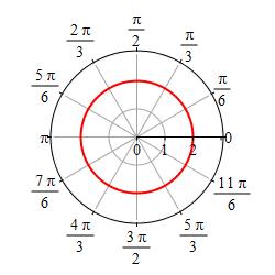
This plot shows a polar coordinate grid labeled with angles in radians.
The circle of radius 2 centered at the origin is drawn.

The graph of \(r=2\) is the set of points \((r,\theta)=(2,\theta)\) for all values of \(\theta\), which is the circle of radius \(2\) centered at the origin.

Graph \(r=\theta\).

We first graph the part of the curve with \(\theta \ge 0\). We start at \(r=\theta=0\) which is the origin. As \(r=\theta\) gets larger, we travel around counterclockwise and the radius also gets larger. So we trace out a spiral as shown in the first plot.

This animation shows a polar grid where a curve comes out of the origin
along the positive x-axis and bends upward and spirals outward
counterclockwise. A dot is moving along the curve out from the origin.

As \(r=\theta\) gets negative, we travel around clockwise and since \(r\) is also negative, we measure \(|r|\) backwards, which traces out a spiral which is the mirror image through the \(y\)-axis of the first half as shown in the second plot.

This animation starts with the same polar grid and curve as above, but
now there is another curve which spirals outward clockwise it is the
mirror image of the first one across the y-axis. A dot is moving along the
curves first inward along the new curve and then outward along the original
curve.

If we restrict to the part of the curve, \(r=\theta\), with \(-\,\dfrac{3\pi}{2} \le \theta \le \dfrac{3\pi}{2}\), we get a heart shape.

Happy Valentine's Day!

This animation shows the parts of the curves from above which form
a symmetric heart shape. The dot moves around on the curve.

Most polar equations, however, are not so transparent! On the next page, we look at successively more complicated functions and successively more refined graphing techniques.

15. Polar Coordinates

b.1. Graphs of Polar Equations

Heading